Merges and Joins: From SQL to Stata

Diagrams and code examples in Sections 1–4 are adapted from:

Wickham H, Çetinkaya-Rundel M, Grolemund G (2023). R for Data Science, 2nd ed., Chapter 19 “Joins”. https://r4ds.hadley.nz/joins.html

That work is licensed under CC BY-NC-ND 3.0. The Stata-specific material in Sections 5–6 is original.

Note

Language coverage: All executable code in Sections 1–4 is R and runs live in this notebook. Equivalent Julia (DataFrames.jl) syntax is shown alongside each example for reference but is not executed. A fully worked, copy-paste-ready Stata example appears in Section 7.

# Loading 2 R libraries to illustrate
library(tidyverse)
library(nycflights13)

1 Keys: the foundation of every join

Every join connects two tables through a pair of keys.

A primary key uniquely identifies each row in a table. It may be a single variable or a compound key (multiple variables together).
A foreign key references the primary key of another table.

In the nycflights13 package, for example, we have tables planes, flights and airlines:

head(select(planes,tailnum,year,model),3)

# A tibble: 3 × 3
  tailnum  year model    
  <chr>   <int> <chr>    
1 N10156   2004 EMB-145XR
2 N102UW   1998 A320-214 
3 N103US   1999 A320-214

and flights

flights |>
  select(tailnum,year,month,day) |>
  arrange(tailnum) |>
  head(3)

# A tibble: 3 × 4
  tailnum  year month   day
  <chr>   <int> <int> <int>
1 D942DN   2013     2    11
2 D942DN   2013     3    23
3 D942DN   2013     3    24

planes$tailnum is the primary key of planes; flights$tailnum is a foreign key pointing to it.
similarly for airlines$carrier, which is the primary key of airlines; flights$carrier is the foreign key.
weather uses the compound primary key (origin, time_hour).

1.1 Always verify key uniqueness

Before joining, check that the variable you intend to use as a key is actually unique on the side where you expect it to be:

planes |>
  count(tailnum) |>
  # any tailnum occuring more than once?
  filter(n > 1) |>
  # Should return 0 rows
  nrow()

[1] 0

# Compound key check
weather |>
  count(time_hour, origin) |>
  # any combo (time,origin) occuring more than once?
  filter(n > 1) |>
  nrow()  # same

[1] 0

Also check for missing values — a missing key cannot identify an observation:

planes |> 
  filter(is.na(tailnum)) |>
  nrow()

[1] 0

Warning

Common mistake: assuming a variable is a unique key without checking. Duplicate keys on the wrong side are the root cause of most unintended many-to-many explosions.

2 How joins work: a visual model

We will use two small tables throughout this section. The key column in x takes values 1, 2, 3; in y it takes values 1, 2, 4. Key 3 exists only in x; key 4 only in y.

# tribble() builds a small data frame row-by-row;
# column names are prefixed with ~ (tilde)
x <- tribble(
  ~key, ~val_x,
     1, "x1",
     2, "x2",
     3, "x3"
)
y <- tribble(
  ~key, ~val_y,
     1, "y1",
     2, "y2",
     4, "y3"
)
x   # print x — 3 rows, keys 1/2/3

# A tibble: 3 × 2
    key val_x
  <dbl> <chr>
1     1 x1   
2     2 x2   
3     3 x3

y   # print y — 3 rows, keys 1/2/4

# A tibble: 3 × 2
    key val_y
  <dbl> <chr>
1     1 y1   
2     2 y2   
3     4 y3

Julia

using DataFrames

x = DataFrame(key = [1, 2, 3], val_x = ["x1", "x2", "x3"])
y = DataFrame(key = [1, 2, 4], val_y = ["y1", "y2", "y3"])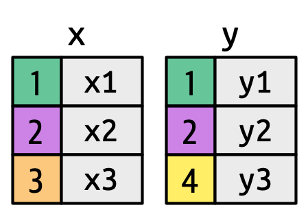

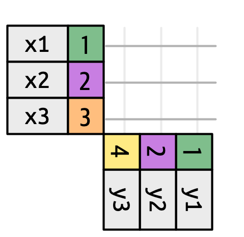
x and y are two data frames with 2 columns and 3 rows. Key values are color-coded. — Two example tables. Key values are color-coded: green=1, purple=2, orange=3, yellow=4.

To reason about any join, imagine a grid of all possible matches between every row of x and every row of y. The join type then determines which intersections become actual rows in the output.

x and y placed at right-angles with a grid of connecting lines showing all potential matches. — Every possible match as a grid. Dots will indicate which intersections produce output rows.

3 The four standard join types

3.1 Inner join

Keeps only rows where the key appears in both tables. Unmatched rows from either side are silently dropped.

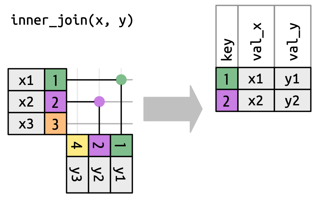
Inner join diagram with dots at key=1 and key=2 intersections. — Inner join: only keys 1 and 2 match, so the output has 2 rows.

x |> inner_join(y, join_by(key))

# A tibble: 2 × 3
    key val_x val_y
  <dbl> <chr> <chr>
1     1 x1    y1   
2     2 x2    y2

Julia

innerjoin(x, y, on = :key)

SQL	Stata	R (dplyr)	Julia (DataFrames.jl)
`INNER JOIN`	`merge …; keep if _merge == 3`	`inner_join()`	`innerjoin()`

3.2 Left join

Keeps all rows from x. Where there is no match in y, value columns from y are filled with NA (Stata: .).

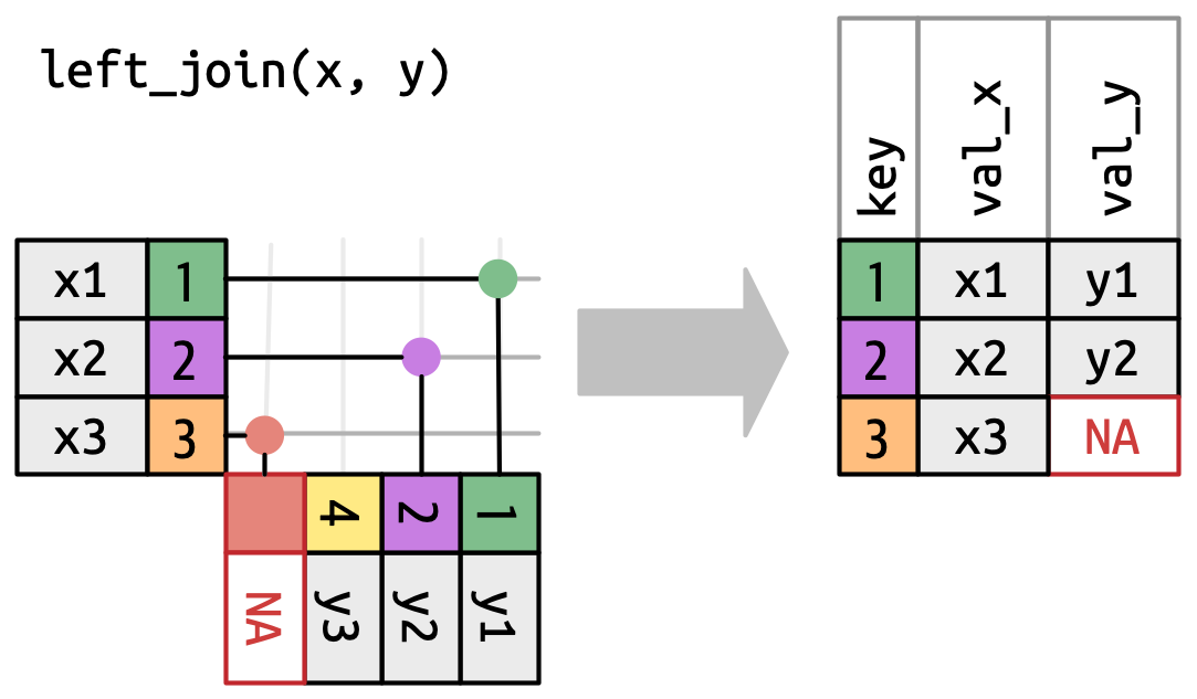
Left join diagram where x gets a virtual row for unmatched key=3. — Left join: all 3 rows of x survive; key=3 gets NA for val_y.

x |> left_join(y, join_by(key))

# A tibble: 3 × 3
    key val_x val_y
  <dbl> <chr> <chr>
1     1 x1    y1   
2     2 x2    y2   
3     3 x3    <NA>

Julia

leftjoin(x, y, on = :key)

SQL	Stata	R (dplyr)	Julia (DataFrames.jl)
`LEFT OUTER JOIN`	`merge …; keep if _merge != 2`	`left_join()`	`leftjoin()`

3.3 Right join

Keeps all rows from y. Unmatched rows from y get NA for the x columns.

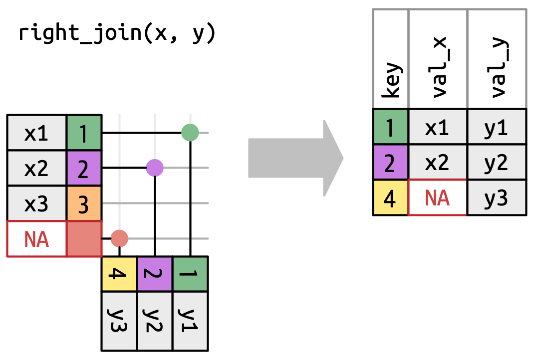
Right join diagram where y gets a virtual row for unmatched key=4. — Right join: all 3 rows of y survive; key=4 gets NA for val_x.

x |> right_join(y, join_by(key))

# A tibble: 3 × 3
    key val_x val_y
  <dbl> <chr> <chr>
1     1 x1    y1   
2     2 x2    y2   
3     4 <NA>  y3

Julia

rightjoin(x, y, on = :key)

SQL	Stata	R (dplyr)	Julia (DataFrames.jl)
`RIGHT OUTER JOIN`	`merge …; keep if _merge != 1`	`right_join()`	`rightjoin()`

3.4 Full join

Keeps all rows from both tables. Unmatched rows get NA on the side with no match. This is Stata’s default merge behavior.

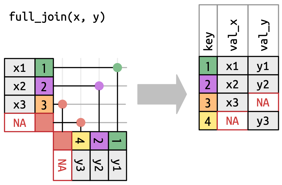
Full join diagram where both x and y have virtual rows for unmatched keys. — Full join: all 4 keys appear; unmatched cells are NA.

x |> full_join(y, join_by(key))

# A tibble: 4 × 3
    key val_x val_y
  <dbl> <chr> <chr>
1     1 x1    y1   
2     2 x2    y2   
3     3 x3    <NA> 
4     4 <NA>  y3

Julia

outerjoin(x, y, on = :key)

SQL	Stata	R (dplyr)	Julia (DataFrames.jl)
`FULL OUTER JOIN`	`merge …` (default, keep all)	`full_join()`	`outerjoin()`

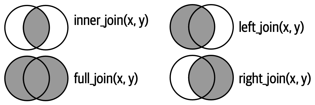
3.5 Venn diagram summary

A useful (though imperfect) memory aid. It correctly shows which rows survive but does not illustrate what happens to columns from the non-surviving side.

Venn diagrams for inner, full, left and right joins showing shaded regions. — Venn diagram view of the four join types.

3.6 Filtering joins

These don’t add columns — they just filter rows based on whether a match exists.

Semi-join: keeps rows in x that have at least one match in y. No columns from y are added.

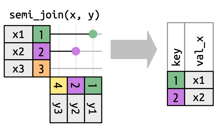
Semi-join diagram showing only matched rows retained from x. — Semi-join: only existence of a match matters.

x |> semi_join(y, join_by(key))

# A tibble: 2 × 2
    key val_x
  <dbl> <chr>
1     1 x1   
2     2 x2

Julia

semijoin(x, y, on = :key)

Anti-join: keeps rows in x that have no match in y. Excellent for diagnosing unmatched observations.

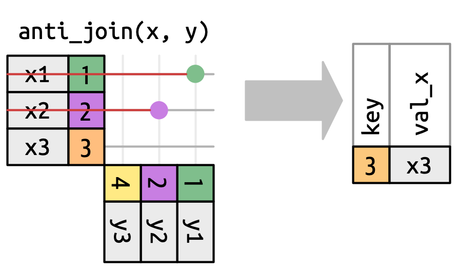
Anti-join diagram where matched rows are marked for dropping. — Anti-join: inverse of semi-join; matched rows are dropped (shown in red).

x |> anti_join(y, join_by(key))

# A tibble: 1 × 2
    key val_x
  <dbl> <chr>
1     3 x3

Julia

antijoin(x, y, on = :key)

4 Row matching and cardinality

What happens when a key value appears more than once on one side?

Join diagram showing key=1 matching once, key=2 matching twice, key=3 matching zero times. — Three matching scenarios: one match, two matches, zero matches.

Three outcomes are possible for a row in x:

Zero matches → dropped (in inner/left joins: kept with NAs for outer joins)
One match → preserved as-is
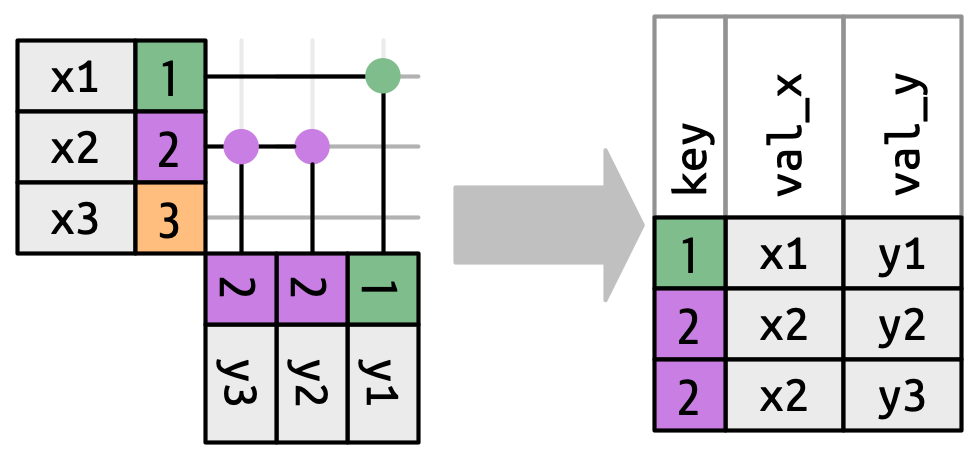
Multiple matches → duplicated once per match

The dangerous case is when both sides have duplicates on the key. With 3 rows for key=2 in x and 3 rows for key=2 in y, a relational join produces 3 × 3 = 9 rows for that key group alone. dplyr warns you:

df1 <- tibble(key = c(1, 2, 2), val_x = c("x1", "x2", "x3"))
df2 <- tibble(key = c(1, 2, 2), val_y = c("y1", "y2", "y3"))

df1 |> inner_join(df2, join_by(key))

Warning in inner_join(df1, df2, join_by(key)): Detected an unexpected many-to-many relationship between `x` and `y`.
ℹ Row 2 of `x` matches multiple rows in `y`.
ℹ Row 2 of `y` matches multiple rows in `x`.
ℹ If a many-to-many relationship is expected, set `relationship =
  "many-to-many"` to silence this warning.

# A tibble: 5 × 3
    key val_x val_y
  <dbl> <chr> <chr>
1     1 x1    y1   
2     2 x2    y2   
3     2 x2    y3   
4     2 x3    y2   
5     2 x3    y3

Key uniqueness	Name	Output rows	Risk
Unique on both sides	1:1	≤ matched rows	Low
Unique on x, duplicates on y	1:m	= rows in y (matched keys)	Low
Duplicates on x, unique on y	m:1	= rows in x (matched keys)	Low
Duplicates on both sides (relational)	m:m	= Cartesian product per group	Verify intent
Stata’s `merge m:m`	positional	= max(n_x, n_y) per group	Critical

5 Stata’s `merge` command

Stata’s merge is a full outer join by default. The _merge indicator it creates tells you the match status of each row:

`_merge` value	Meaning	SQL analogy
`1` — master only	Row in left dataset, no match in right	Left outer, unmatched
`2` — using only	Row in right dataset, no match in left	Right outer, unmatched
`3` — matched	Row matched in both datasets	Inner join result

The merge type prefix declares the expected key cardinality. Stata will error if the data violates the declared cardinality — which is a useful safeguard:

* 1:1 — key unique on BOTH sides
merge 1:1 firm_id year using "balance_sheet.dta"

* m:1 — key may repeat in master, unique in using
*       (adding region-level attributes to a firm-year panel)
merge m:1 region_id using "region_controls.dta"

* 1:m — unique in master, may repeat in using
merge 1:m firm_id using "patents.dta"

* Controlling what rows to keep after the merge
keep if _merge == 3   // inner join
keep if _merge != 2   // left join
keep if _merge != 1   // right join
drop _merge           // always drop _merge when done

Tip

Best practice: always inspect _merge after every merge. Use assert _merge == 3 if you expect a perfect match, or tab _merge to check for unexpected non-matches. Never leave _merge in the working dataset without examining it.

6 The `merge m:m` problem

merge m:m is not a relational join

Despite the name, merge m:m in Stata does not produce the Cartesian product of matching key groups. It performs positional row-matching within key groups: it pairs rows by their position after sorting by the key variable — 1st row with 1st row, 2nd with 2nd, and so on.

This is almost certainly not what the author intended, and its output depends silently on the sort order of the data.

6.1 A concrete example

Suppose both datasets have multiple rows for firm_id = 42:

Master (employees.dta):

firm_id	employee
42	Alice
42	Bob
42	Carol

Using (contracts.dta):

firm_id	contract
42	C-001
42	C-002
42	C-003

6.1.1 What `merge m:m` actually produces

Stata pairs by position within the key group:

merge m:m firm_id using "contracts.dta"

firm_id	employee	contract	How?
42	Alice	C-001	1st ↔︎ 1st
42	Bob	C-002	2nd ↔︎ 2nd
42	Carol	C-003	3rd ↔︎ 3rd

Alice is matched to C-001 not because of any meaningful relationship between them, but because both happen to be first in their respective files. Re-sort either dataset before the merge and you get a different result.

6.1.2 What a true m:m (relational) join produces

joinby in Stata, or inner_join() in R when both sides have duplicates, produces the full Cartesian product — every combination:

firm_id	employee	contract
42	Alice	C-001
42	Alice	C-002
42	Alice	C-003
42	Bob	C-001
42	Bob	C-002
42	Bob	C-003
42	Carol	C-001
42	Carol	C-002
42	Carol	C-003

Nine rows, not three. The merge m:m result is neither a relational join nor a documented data transformation — it is a positional artifact.

6.2 Why this is a critical reproducibility issue

Important

The output of merge m:m is sort-order dependent. Two researchers running the same code on data with different sort histories may get different results — even with identical _merge == 3 counts. The code is logically wrong even when results happen to replicate.

7 Worked Stata example: `merge m:m` vs `joinby`

The script below is self-contained and copy-paste ready: it builds the datasets from scratch using input, runs both the wrong and the correct merge, and cleans up after itself. No external .dta files are needed.

7.1 Step 1 — Build the two datasets

clear all
set more off

* --- employees.dta -----------------------------------------------------------
input str10 firm_id str8 employee
    "firm_42"   "Alice"
    "firm_42"   "Bob"
    "firm_42"   "Carol"
    "firm_99"   "Dave"
end

label var firm_id  "Firm identifier"
label var employee "Employee name"

save employees.dta, replace

* --- contracts.dta -----------------------------------------------------------
clear
input str10 firm_id str8 contract
    "firm_42"   "C-001"
    "firm_42"   "C-002"
    "firm_42"   "C-003"
    "firm_99"   "D-001"
end

label var firm_id  "Firm identifier"
label var contract "Contract reference"

save contracts.dta, replace

7.2 Step 2 — The wrong way: `merge m:m`

Stata pairs rows by position within each key group after sorting. The result depends entirely on the current sort order of both files — it is not a relational join.

use employees.dta, clear

display as text _newline ///
    "================================================" _newline ///
    "  WRONG: merge m:m (positional row-pairing)"     _newline ///
    "================================================"

merge m:m firm_id using contracts.dta

* Alice→C-001, Bob→C-002, Carol→C-003 — purely positional.
* Re-sort either file and you get different pairs.
list firm_id employee contract _merge, sepby(firm_id) noobs


  +---------------------------------------------+
  | firm_id   employee   contract        _merge |
  |---------------------------------------------|
  | firm_42      Alice      C-001   Matched (3) |
  | firm_42        Bob      C-002   Matched (3) |
  | firm_42      Carol      C-003   Matched (3) |
  |---------------------------------------------|
  | firm_99       Dave      D-001   Matched (3) |
  +---------------------------------------------+


* All _merge == 3 gives false confidence that the merge "worked"
tab _merge

   Matching result from |
                  merge |      Freq.     Percent        Cum.
------------------------+-----------------------------------
            Matched (3) |          4      100.00      100.00
------------------------+-----------------------------------
                  Total |          4      100.00

7.3 Step 3 — Demonstrating sort-order dependence

* Reverse the order of contracts for firm_42 and re-run.
* The employee-contract pairs change — even though _merge is still all 3s.

use contracts.dta, clear
gsort firm_id -contract          // reverse alphabetical order within firm
save contracts_reversed.dta, replace

use employees.dta, clear

display as text _newline ///
    "================================================"         _newline ///
    "  WRONG: merge m:m after reversing contracts"             _newline ///
    "  (same _merge=3, completely different pairs!)"           _newline ///
    "================================================"

merge m:m firm_id using contracts_reversed.dta

* Now Alice→C-003, Bob→C-002, Carol→C-001
* The 'result' changed just because we re-sorted the using file.
list firm_id employee contract _merge, sepby(firm_id) noobs

  +---------------------------------------------+
  | firm_id   employee   contract        _merge |
  |---------------------------------------------|
  | firm_42      Alice      C-003   Matched (3) |
  | firm_42        Bob      C-002   Matched (3) |
  | firm_42      Carol      C-001   Matched (3) |
  |---------------------------------------------|
  | firm_99       Dave      D-001   Matched (3) |
  +---------------------------------------------+

7.4 Step 4 — The right way: `joinby`

joinby produces the true relational many-to-many join: the full Cartesian product within each key group. Every (employee, contract) combination appears exactly once, and the result does not depend on sort order.

use employees.dta, clear

display as text _newline ///
    "================================================" _newline ///
    "  CORRECT: joinby (Cartesian product per group)" _newline ///
    "================================================"

joinby firm_id using contracts.dta

list firm_id employee contract, sepby(firm_id) noobs

  +-------------------------------+
  | firm_id   employee   contract |
  |-------------------------------|
  | firm_42      Alice      C-002 |
  | firm_42      Alice      C-001 |
  | firm_42      Alice      C-003 |
  | firm_42        Bob      C-002 |
  | firm_42        Bob      C-003 |
  | firm_42        Bob      C-001 |
  | firm_42      Carol      C-001 |
  | firm_42      Carol      C-003 |
  | firm_42      Carol      C-002 |
  |-------------------------------|
  | firm_99       Dave      D-001 |
  +-------------------------------+


* firm_42: 3 employees × 3 contracts = 9 rows  ✓
* firm_99: 1 employee  × 1 contract  = 1 row   ✓

7.5 Step 5 — What you probably actually wanted: `merge 1:1` with a proper key

In most real cases, merge m:m signals a missing key variable. The data likely has a meaningful unique key you haven’t identified yet. Once you find it, use the appropriate typed merge:

* employees with explicit contract assignment
clear
input str10 firm_id str8 employee str8 contract_id
    "firm_42"   "Alice"   "C-001"
    "firm_42"   "Bob"     "C-002"
    "firm_42"   "Carol"   "C-003"
    "firm_99"   "Dave"    "D-001"
end
save employees_with_key.dta, replace

clear
input str10 firm_id str8 contract_id str20 contract_desc
    "firm_42"   "C-001"   "Software license"
    "firm_42"   "C-002"   "Consulting retainer"
    "firm_42"   "C-003"   "Hardware supply"
    "firm_99"   "D-001"   "Maintenance contract"
end
save contracts_with_key.dta, replace

use employees_with_key.dta, clear

display as text _newline ///
    "================================================"          _newline ///
    "  ALTERNATIVE: merge 1:1 once you identify the key"        _newline ///
    "================================================"

merge 1:1 firm_id contract_id using contracts_with_key.dta

list firm_id employee contract_id contract_desc _merge, sepby(firm_id) noobs

  +--------------------------------------------------------------------+
  | firm_id   employee   contra~d          contract_desc        _merge |
  |--------------------------------------------------------------------|
  | firm_42      Alice      C-001       Software license   Matched (3) |
  | firm_42        Bob      C-002    Consulting retainer   Matched (3) |
  | firm_42      Carol      C-003        Hardware supply   Matched (3) |
  |--------------------------------------------------------------------|
  | firm_99       Dave      D-001   Maintenance contract   Matched (3) |
  +--------------------------------------------------------------------+


assert _merge == 3   // all rows should match — error if not

7.6 Clean up

erase employees.dta
erase employees_with_key.dta
erase contracts.dta
erase contracts_reversed.dta
erase contracts_with_key.dta

display as text _newline "Done."

Command	Semantics	Output rows	Use when
`merge 1:1`	Relational, unique key both sides	≤ rows in master	Adding scalar attributes
`merge m:1`	Relational, unique key on using side	= rows in master	Adding group-level vars to panel
`merge 1:m`	Relational, unique key on master side	≥ rows in master	Expanding (e.g. firm → firm-product)
`joinby`	True m:m Cartesian join	= product of group sizes	Rarely; only when all combos are meaningful
`merge m:m`	Positional row-pairing ⚠️	= max(n_x, n_y) per group	Almost never

8 Quick reference

SQL	Stata	R (dplyr)	Julia (DataFrames.jl)	Rows kept
`INNER JOIN`	`merge …; keep if _merge==3`	`inner_join()`	`innerjoin()`	Both sides matched
`LEFT OUTER JOIN`	`merge …; keep if _merge!=2`	`left_join()`	`leftjoin()`	All of master
`RIGHT OUTER JOIN`	`merge …; keep if _merge!=1`	`right_join()`	`rightjoin()`	All of using
`FULL OUTER JOIN`	`merge …` (default)	`full_join()`	`outerjoin()`	All rows both sides
`WHERE EXISTS`	—	`semi_join()`	`semijoin()`	x rows with a match in y
`WHERE NOT EXISTS`	—	`anti_join()`	`antijoin()`	x rows with no match in y
Cartesian m:m	`joinby`	(dplyr warns, use `relationship="many-to-many"`)	`crossjoin()`	All combinations
⚠️ Positional pairing	`merge m:m`	—	—	Unpredictable — avoid

Tip

Pre-merge checklist:

Run duplicates report [keyvar] on both datasets.
Choose the merge type that matches the actual cardinality.
After merging, always inspect _merge — never leave it unchecked.
Assert the expected outcome: assert _merge == 3 if all rows should match.
If you find merge m:m in someone else’s code: flag it.

9 Further reading

Wickham H, Çetinkayer-Rundel M, Grolemund G (2023). R for Data Science (2e), Ch. 19 Joins. https://r4ds.hadley.nz/joins.html
Stata manual: help merge, help joinby
StataCorp (2023). Stata Base Reference Manual, merge entry — note the explicit warning against merge m:m

1 Keys: the foundation of every join

1.1 Always verify key uniqueness

2 How joins work: a visual model

3 The four standard join types

3.1 Inner join

3.2 Left join

3.3 Right join

3.4 Full join

3.5 Venn diagram summary

3.6 Filtering joins

4 Row matching and cardinality

5 Stata’s merge command

6 The merge m:m problem

6.1 A concrete example

6.1.1 What merge m:m actually produces

6.1.2 What a true m:m (relational) join produces

6.2 Why this is a critical reproducibility issue

7 Worked Stata example: merge m:m vs joinby

7.1 Step 1 — Build the two datasets

7.2 Step 2 — The wrong way: merge m:m

7.3 Step 3 — Demonstrating sort-order dependence

7.4 Step 4 — The right way: joinby

7.5 Step 5 — What you probably actually wanted: merge 1:1 with a proper key

7.6 Clean up

8 Quick reference

9 Further reading

5 Stata’s `merge` command

6 The `merge m:m` problem

6.1.1 What `merge m:m` actually produces

7 Worked Stata example: `merge m:m` vs `joinby`

7.2 Step 2 — The wrong way: `merge m:m`

7.4 Step 4 — The right way: `joinby`

7.5 Step 5 — What you probably actually wanted: `merge 1:1` with a proper key